An animation of a vibrating building looks continuous and smooth. A computer, however, divides time into short intervals and predicts motion step by step. If each step makes the vibration slightly faster or slower, the accumulated error shifts the peaks away from their true timing.
Getting the rhythm right, not just the amplitude
A time-integration algorithm advances the structural equations of motion to the next instant. Researchers assess whether the calculation remains stable, whether amplitudes undergo artificial decay, and whether vibration periods become longer or shorter. The last type of error is commonly called numerical dispersion.
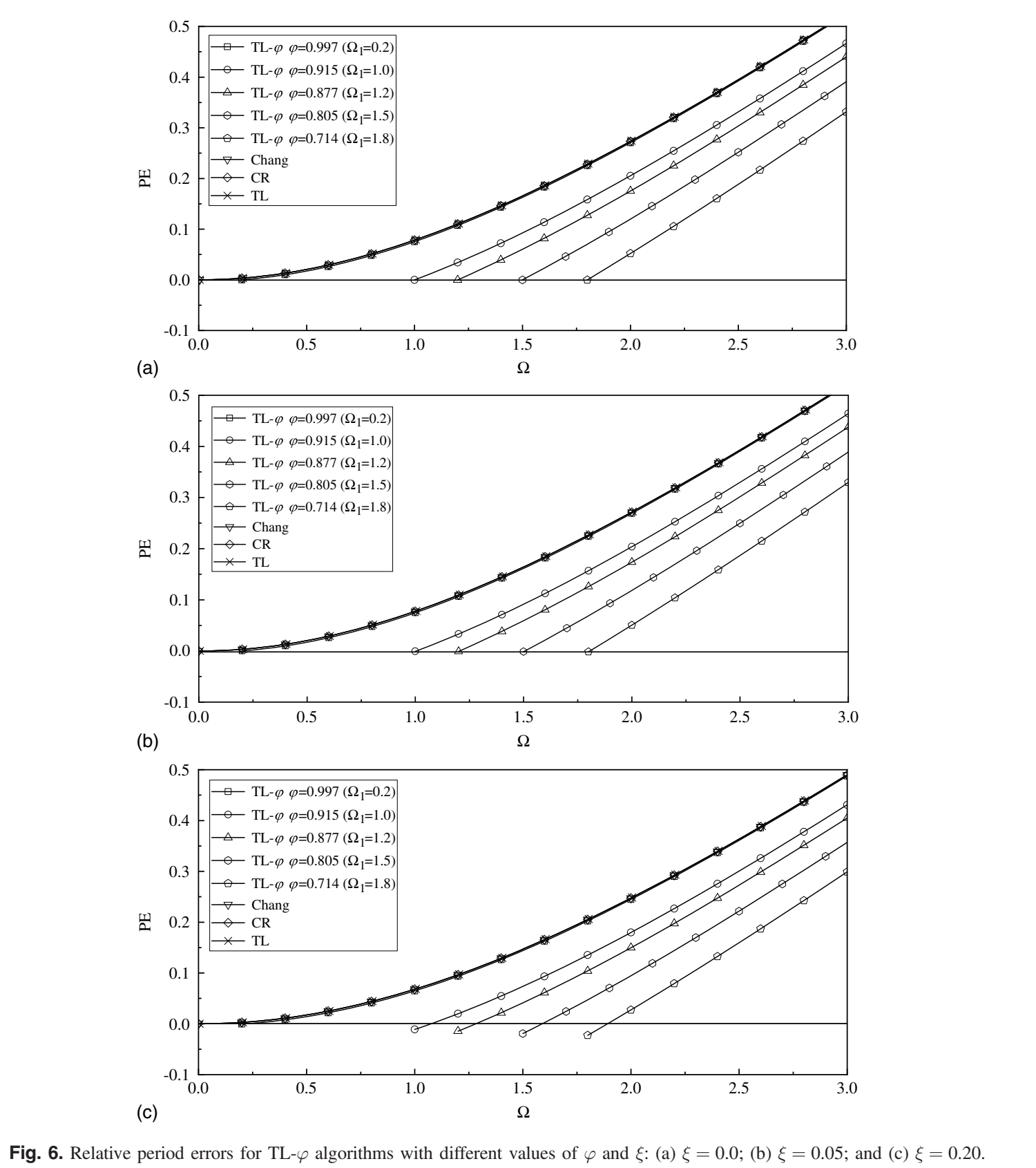
This paper introduces the TL-φ family of explicit algorithms with controllable numerical dispersion. Using the structure's own dynamic properties, the parameter φ adjusts period error so that the calculated motion follows the original rhythm more closely over the frequency range of interest. The curves illustrate this tuning capability.
Explicit describes how the next state is computed: the algorithm uses information already available to advance directly, making it useful for dynamic analyses with many time steps. Structure-dependent means that its coefficients depend on the dynamic characteristics of the structure being analysed. Drawing on transformations from control theory, the paper aligns the algorithm's vibration characteristics more closely with those of the target system. The parameter φ acts like a calibration knob for the rhythm of motion in discrete time.
Zoom in to see whether the peaks line up
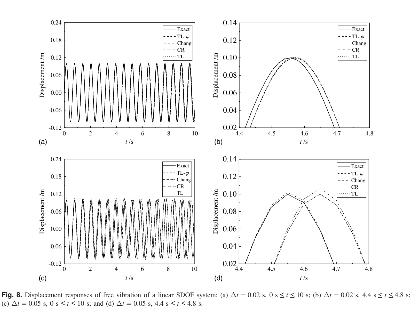
The paper compares algorithms using several linear and nonlinear examples. Curves may look similar over a complete time history, but zooming into one oscillation reveals whether a peak arrives early or late. The enlarged views on the right make these differences easy to recognize.
A larger time step spans more motion in each update, allowing period error to accumulate more readily. An appropriate φ value can improve this deviation while having relatively little effect on other algorithmic properties. This is particularly useful when waveform and response phase matter.
The upper and lower sets in the figure use different time steps. With the smaller step, many curves lie close together; with the larger step, the misalignment of local peaks becomes clearer. Even a small error per cycle can accumulate into a visible phase difference after many oscillations. For a single response peak, this changes when the maximum occurs. In a multi-degree-of-freedom structure, it also affects whether motions at different locations combine at the correct time.
Match the time step to the structure
The study discusses stability conditions for linear and nonlinear systems separately. The linear system has unconditional stability, while nonlinear analysis still requires parameters selected according to the relevant conditions. Stability and accuracy have different jobs: a calculation that runs successfully must still be checked for correct amplitude and period.
The work adds an adjustable control to time integration. Understanding the structure's main vibration rhythms and choosing the algorithm and time step accordingly can make the simulated motion more faithful to the motion being studied.
Examples of increasing complexity extend validation from a regular single oscillator to multi-degree-of-freedom and nonlinear systems. Time-step selection can begin with the frequency range that must be represented accurately, followed by checks of period error and amplitude changes. Algorithm parameters then become tied to the task: interest in slow overall sway or in faster local motion determines where accuracy should be concentrated.