Real seismic waves travel through vast expanses of ground. A computer model always has boundaries: usually we retain only a region around a bridge, tunnel or site. How to bring distant earthquake waves into that region, while allowing outgoing waves to leave, is a fundamental problem in numerical simulation.
Bring a distant earthquake to the model boundary
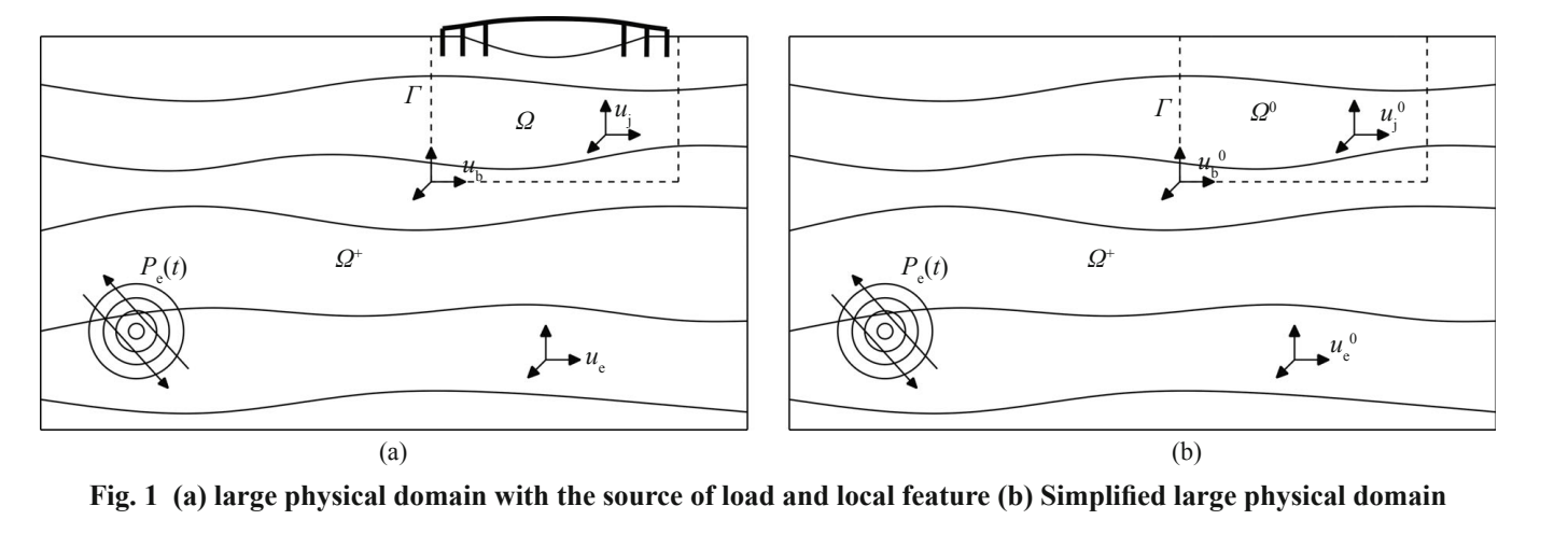
The domain reduction method offers one solution: first calculate waves in a larger, relatively simplified site, then convert those motions into equivalent loads near the boundary of the local model. The local model can retain complex terrain and structural details while receiving the external wave field through its boundary.
The dashed box in the figure identifies the region requiring detailed study. Building on the original domain reduction method, the paper includes damping-related terms in the equivalent input to form a modified method. Damping describes a material's ability to dissipate energy during motion, so it also affects the actions that should be applied at the boundary.
This divides a large problem into two steps: establish how the distant earthquake propagates through simpler geology, then investigate what happens when the waves enter a complex local region. The first step supplies free-field motion; the second allows terrain, soil layers and structures to generate scattered waves. Equivalent loads connect the two, transferring the external field's action along an enclosing region to the local model. A more accurate connection keeps the detailed calculation consistent with its regional background.
A small detail changes the vertical waveform
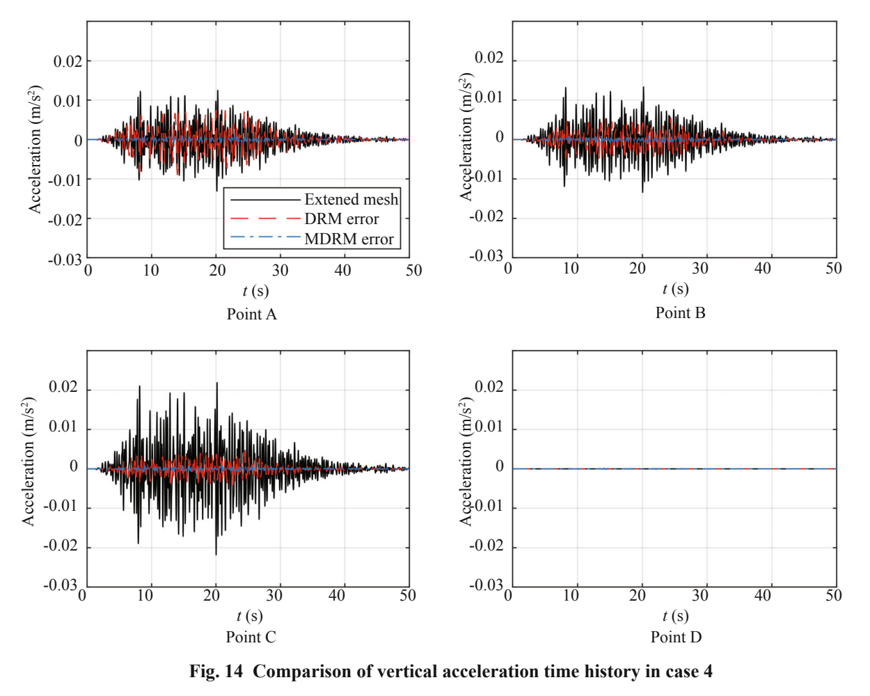
The study uses several wave-propagation examples, with a larger model as the reference, to compare acceleration histories. Both the original and modified methods perform well for horizontal response. Vertical response more readily exposes differences in the treatment of damping.
Under one set of validation conditions, the modified method substantially reduces vertical acceleration error. In the original figure, the black curve is the extended-model response, while red and blue show errors from the two methods. Focus on the error curves near zero: smaller errors indicate that the local model reproduces the external wave field more accurately.
Differences are easier to see in the weaker vertical response. Horizontal waves interacting with local terrain can generate vertical motion, whose amplitude and phase depend on how the model handles this coupling. The damping contribution omitted by the original method can become a noticeable source of error at certain times. Including it changes the distance of the red and blue error curves from zero. This represents improved input-transfer accuracy, not additional energy in the real earthquake.
Boundary position matters too
Even with the input formula corrected, waves still need sufficient space to propagate. If an artificial boundary is too close, reflected waves may re-enter the region of interest and affect the results. The paper therefore also examines the relationship between boundary distance and error.
The work connects a finite computational domain more accurately to earthquake motion in a much larger site. For projects requiring detailed local terrain and structural models, this helps concentrate computational resources where they are most useful.
Boundary checks can compare not only maxima but also peaks and troughs throughout the history, duration, and the return to a steady state. Extra reflections at model edges often reach observation areas later, so simulation duration and boundary distance must be considered together. Examples with different distances and inputs link two questions—where to place the boundary and what to apply there—into a fuller validation strategy for local seismic analysis.